Some smart readers wrote saying that they are familiar with R but not the microbiome. This post is intended to kickstart them on a simple desired goal:

Which bacteria (or combination of bacteria) are associated with certain symptoms.

We have 240 symptoms and thousands of bacteria … oops, a big problem. We do not have a lot of microbiomes with symptoms list — so we are likely forced to deal with only the most common symptoms at present.

Information about bacteria is layered

A quick read on wikipedia on bacteria taxonomy may help. If you just grab the Taxonomy file, you will see the species counted in with it’s parent genus, who is counted in with family, etc… not the best scenario for analysis.

To simplify out matters, I have done extracts on each layer and dropped them at http://lassesen.com/ubiome/

So to load one layer, it’s just a few lines

library(tidyverse)
Species <-read_csv(“http://lassesen.com/ubiome/TaxonomyByspecies.csv&#8221;)
symptoms <-read_csv(“http://lassesen.com/ubiome/Symptoms.csv&#8221; )
samplesymptom <-read_csv(“http://lassesen.com/ubiome/SampleSymptom.csv&#8221;)
samplesWithTitle <- inner_join(samplesymptom, symptoms, by=”symptomId” )

Looking at this one, we find some 2,181 columns (species) and a sampleId (that matches that in symptoms).

From my prior post, you can see how we can get the most common symptom (symptomId=1,”General: Fatigue”) and then a list of sampleId with:

HasFatigue <-samplesWithTitle %>% filter(symptomId==1)

We need to only include observations that reported ANY symptoms, which is easy to do:

PeopleWithSymptoms <- samplesymptom %>% group_by(sampleId) %>% summarize(peopleWith=n()) %>% arrange(peopleWith)

Next we joins this with the level of taxonomy we wish to explore.

SpeciesWithSymptoms <-merge(PeopleWithSymptoms ,Species, by=”sampleId”)

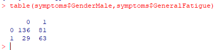
We next put the sets together and set symptomId to 0 for those without fatigue. We have 47.5% of the records with Fatigue.

fulldata <- left_join(SpeciesWithSymptoms,HasFatigue,by=”sampleId”)
fulldata$symptomId =ifelse(is.na(fulldata$symptomId),0,fulldata$symptomId)
#We need to remove the symptom_name
drops <- c(“symptom_name”)
regdata <-fulldata[, !(names(fulldata) %in% drops)]

Picking the Model

I went with a simple linear model for the sake of illustration and toss everything at it!

test <- lm(symptomId ~ .,regdata)

We end up getting a rather long report back:

Where there is a + sign, it indicates increased risk of fatigue as the numbers of bacteria increases, -sign decreased risk of fatigue as the numbers of bacteria increases.

I can now redo it, picking just a few bacteria:

and then looking at the statistics, we see that there is no statistical significance for this relationship (we want to see a p-value < 0.001)

That’s it. No revelations — just an illustration of walking the path. All of the code for above is below.

library(tidyverse)
Species <-read_csv(“http://lassesen.com/ubiome/TaxonomyByspecies.csv&#8221;) symptoms <-read_csv(“http://lassesen.com/ubiome/Symptoms.csv&#8221; ) samplesymptom <-read_csv(“http://lassesen.com/ubiome/SampleSymptom.csv&#8221;) samplesWithTitle <- inner_join(samplesymptom, symptoms, by=”symptomId” ) HasFatigue <-samplesWithTitle %>% filter(symptomId==1)
PeopleWithSymptoms <- samplesymptom %>% group_by(sampleId) %>% summarize(peopleWith=n()) %>% arrange(peopleWith)
SpeciesWithSymptoms <-merge(PeopleWithSymptoms ,Species, by=”sampleId”)

fulldata <- left_join(SpeciesWithSymptoms,HasFatigue,by=”sampleId”)
fulldata$symptomId =ifelse(is.na(fulldata$symptomId),0,fulldata$symptomId)
drops <- c(“symptom_name”)
regdata <-fulldata[, !(names(fulldata) %in% drops)]
test <- lm(symptomId ~ .,regdata)

Doing a run with Phylum,

Phylum <-read_csv(“http://lassesen.com/ubiome/TaxonomyByPhylum.csv&#8221;) symptoms <-read_csv(“http://lassesen.com/ubiome/Symptoms.csv&#8221; ) samplesymptom <-read_csv(“http://lassesen.com/ubiome/SampleSymptom.csv&#8221;) samplesWithTitle <- inner_join(samplesymptom, symptoms, by=”symptomId” ) HasFatigue <-samplesWithTitle %>% filter(symptomId==1)
PeopleWithSymptoms <- samplesymptom %>% group_by(sampleId) %>% summarize(peopleWith=n()) %>% arrange(peopleWith)
PhylumWithSymptoms <-merge(PeopleWithSymptoms ,Phylum, by=”sampleId”)
fulldata <- left_join(PhylumWithSymptoms,HasFatigue,by=”sampleId”)
fulldata$symptomId =ifelse(is.na(fulldata$symptomId),0,fulldata$symptomId)
drops <- c(“symptom_name”)
regdata <-fulldata[, !(names(fulldata) %in% drops)]
test <- lm(symptomId ~ .,regdata)

We find statistical significance with 45% explained by the phylum.

I just received my uBiome report for a sample taken 6 days after a sudden onset ME flare. It was sudden onset because over 15 minutes I could feel my entire body shift and booked off sick for the rest of that day (and following week). The cause was stress, the cause of 40% of ME cases according to studies (the other 60% were infections).

I have two normal health ubiome for reference (each at least 6 months apart). As you can see with this first chart, three important groups did a nose dive.

This is repeated with other groups:

Other items are unchanged, such as diversity

And looking at various levels of bacteria, nothing jumps out

Microbiome Site Analysis

I uploaded the JSON to
http://microbiomeprescription.com/upload , and then look at various reports.

What shows up in the comparison is that High Counts across all conditions went up by 30%.

Some specific jumps:

In terms of the experimental End Produces, we also see some interesting shifts (most numbers were roughly the same)

Large drops in following genus (was normal-range earlier and often went down to -98%)

• Akkermansia
• Anaerococcus
• Dialister
• Enterobacter
• Porphyromonas
• Staphylococcus
• Succiniclasticum

Major increases in following genus:

• Prevotella
• Thalassospira

Bottom Line

First item is that this is likely a unique report — 6 days after onset. A diagnosis of ME/CFS classically requires 6 months of extensive no-results testing, so any ubiome test result would be after a significant progression of microbiome shifts.

Lactic acid producers has crashed, histamine and hydrogen peroxide producers have increased. Significant shift towards a IBS/IBD profile.

Probiotics

After preparing this post, I started with Enterogermina (4 Bacillus clausii in suspension) and within 12 hours found significant changes including:

• Stopping high frequency stool movements that had been ongoing for 4 days
• Change of mood – from borderline depression to very mellow and very very laid back.

It was interesting to note the list of avoid

Plans going forward (reduce the high ones)

• berberine (unfortunately if decrease one high, and increases the other — but it is the only substance know to reduce thalassospira)
• melatonin supplement
• mastic gum (prebiotic)

One of the items, choline deficiency, means that I should cut out my usual 2 eggs each morning because they are high in choline.

Some of the strong avoids were interesting (and unexpected)

We will continue onwards from my last post . Our first step is to determine how many clusters (groupings) of the symptoms that our current data supports.

We do this by trying every size up to 25 and then inspect the chart. The first part is pretty standard R code.

symptoms <-read_csv(“http://lassesen.com/ubiome/SymptomsObservations.csv&#8221;) scaled=scale(symptoms) par(mfrow = c(1, 1)) wss <-0 for (i in 1:25) { km.out <- kmeans(scaled, centers = i, nstart = 20, iter.max = 50) wss[i] <- km.out$tot.withinss }

We then go and drop this data on a plot:

plot(1:25, wss, type = “b”, main=”Ability to decompose symptoms”, xlab = “Number of Clusters”, ylab = “Within groups sum of squares”)

The chart indicate that we likely only have two clusters that are distinct. While our hope was to be able to better cluster people by their symptoms — there is just not enough data yet.

We can look at just 2 clusters with this code

km.out <- kmeans(scaled, centers = 2,nstart = 20, iter.max = 50) km.out

This gives us a list(km.out$cluster) showing which symptom belongs to which group. We then compute the average (mean) for each group and each symptom. We then do some manipulation to change the structure of the table so we get symptom, average in Group1, average in Group 2.

symptoms$cluster=km.out$cluster
group1 <-aggregate(symptoms, by=list(symptoms$cluster),mean) %>% gather(symptom,group,-cluster) %>% filter(cluster==1)
group2 <-aggregate(symptoms, by=list(symptoms$cluster),mean) %>% gather(symptom,group,-cluster) %>% filter(cluster==2)
colnames(group2) = c(“c”,”symptom”,”group2″) colnames(group1) = c(“c”,”symptom”,”group1″) report<-merge(group1,group2,by=”symptom”) %>% select(symptom,group1,group2)
report

We can then sort the symptoms by the differences between group:

report %>% arrange(desc(group2-group1))

For symptoms that do not vary much between the groups we see a lot of official diagnosis that are not ME/CFS like –

Building a model for ME/CFS only

The above was done for ALL samples uploaded — a mixed bag. As see, we could classify by symptoms into a ME/CFS group (Group 2) and a non ME/CFS group (Group 1).

With the above R-Scripts we can apply it to a subset that we define by selecting one or more symptoms as being required. For ME/CFS: GeneralFatigue.

And the same code as above

Again the chart suggests that two clusters is what the data supports.

Create the report, as above:

And now the symptoms that MOST separate the groups. We see that one group was various symptoms — having any would drop them into Group 1.

Looking at what least separate we see a lot of symptoms with no observations that also had general fatigue. Many of these symptoms are associated with ME/CFS — This implies that the picking of
general fatigue alone, was likely a bad choice.

BOTTOM LINE

This post intent was NOT to discover an interesting fact, but to show how you can explore the data (and hopefully discover an interesting fact that you will share).

To make your life easier, I have the R code needed below to do your investigations.

library(tidyverse)
symptoms <-read_csv(“http://lassesen.com/ubiome/SymptomsObservations.csv&#8221;) meSymptoms <- symptoms %>% filter([YOUR ITEM 1]==1,[YOUR ITEM 2]==1)
dim(meSymptoms) #see how many rows you have

par(mfrow = c(1, 1))
wss <-0
for (i in 1:25) {
# Fit the model: km.out
km.out <- kmeans(meSymptoms, centers = i, nstart = 20, iter.max = 50)
# Save the within cluster sum of squares
wss[i] <- km.out$tot.withinss
}
plot(1:25, wss, type = “b”, main=”Ability to decompose ME symptoms”,
xlab = “Number of Clusters”,
ylab = “Within groups sum of squares”)

meSymptoms$cluster=km.out$cluster
group1 <-aggregate(meSymptoms, by=list(meSymptoms$cluster),mean) %>% gather(symptom,group,-cluster) %>% filter(cluster==1)
group2 <-aggregate(meSymptoms, by=list(meSymptoms$cluster),mean) %>% gather(symptom,group,-cluster) %>% filter(cluster==2)
colnames(group2) = c(“c”,”symptom”,”group2″)
colnames(group1) = c(“c”,”symptom”,”group1″)
report<-merge(group1,group2,by=”symptom”) %>% select(symptom,group1,group2)
report %>% arrange(desc(abs(group2-group1))) #most different
report %>% arrange(abs(group2-group1)) #least different

Caution

When the number of observations go low, you may get no meaningful results. Example:

We expect to see a big drop initially and then a clear “elbow” in the curve. There was none appearing with the above.

You may wish to read my prior post here to get a framework for this post. This is intended to get readers to play with the data with some simple canned queries.

There are two ways to view symptom data this

• Classic R (nerd) way – tidying data and dealing with n/a
• Using a prepared CSV file that is ready to go

Classic way

The following lines will create the data.frames to work with

• library(tidyverse)
• symptoms <-read_csv(“http://lassesen.com/ubiome/Symptoms.csv&#8221; )
• samplesymptom <-read_csv(“http://lassesen.com/ubiome/SampleSymptom.csv&#8221;)
• samplesWithTitle <- inner_join(samplesymptom, symptoms, by=”symptomId”)

This allows some queries but also exposes challenges with converting symptom_names to column names. I will leave things for R-nerds and proceed to the alternative method.

samplesWithTitle %>% group_by(symptomId,symptom_name) %>% summarize(peopleWith=n()) %>% arrange(desc(peopleWith))

Transformed Data

One of my exports addresses the challenges of symptoms names by removing awkward characters such as (‘,:,).

symptoms <-read_csv(“http://lassesen.com/ubiome/SymptomsObservations.csv&#8221;)

To see all of the symptom (column) names – a total of 240 of them!

colnames(symptoms)

Simple Tables

We can get information about any combination of columns. 1 means true (checked) 0 means false (not checked), for example

One problem is that not everyone gave their gender. To make life easier, we can create a new column, “Sex” with this little bit of code. Note that the values are 1 (TRUE) and 0 (FALSE), so we do not need to write ”
symptoms$GenderMale ==1″, instead just “symptoms$GenderMale”

symptoms$sex = ifelse(symptoms$GenderMale,”M”,ifelse(symptoms$GenderFemale,”F”,”U”))

Now we see things better

We can do the same thing for blood types, i.e.

symptoms$blood_type <- ifelse(symptoms$BloodTypeANegative,”a-“,
ifelse(symptoms$BloodTypeOPositive,”o+”,
ifelse(symptoms$BloodTypeAPositive,”a+”,”U”)))

One of the problems with our data is that often only a few persons provided data. We cannot conclude that only females are o+.

Finding Relationships

Next we are going to look at what groups of symptoms are clustered together. To be more precise — which patients have similar symptoms and thus could be deemed to be a class. This is done by a technique called clustered analysis. This is done by three different method (Complete, Average, Simple). Complete is the recommended approach.

To simplify the code we reload the data and do not add extra columns such as sex or blood type. The lines below computes the normalized distances between every symptoms with each other (240 x 240 computations)

library(tidyverse)

symptoms2 <-read_csv(“http://lassesen.com/ubiome/SymptomsObservations.csv&#8221;)

symptoms.scaled <-dist(scale(symptoms2))

Hierarchical Clustering – Complete

We are clustering people with similar symptoms together and end up with three interesting charts. The charts are on the same data but done in different ways. The number shown on the chart is the observation(person) number in our data.

symptoms.complete <-hclust(symptoms.scaled,method=”complete”)

plot(symptoms.complete)

Note that the numbers on the left is the distance that one person is from the next one (shown by the line length).

Patient #47 is sitting by themselves. If you want to see what this person symptoms is, then just enter “str(transpose(symptoms2[47,]))” which will show #47 symptoms (we see that there is a massive number of them – which may be why they are off by themselves)

symptoms.average <-hclust(symptoms.scaled,method=”average”)

plot(symptoms.average, main=”Patients symptoms using average Distance”)

symptoms.single <-hclust(symptoms.scaled,method=”single”)

plot(symptoms.single)

Reader Playground

The above is a high level “how to do it”. If you want to look only at how a certain group of symptoms are clustered, then it is simple, just add the symptoms you have (you can be explicit in the symptoms you don’t have by using “gender__female == 0”

mysymptoms <- filter(symptoms2, GenderMale, GeneralDepression)

dim(mysymptoms)

we see just 24 rows (other people) and 240 symptoms

Now, let us see what are the odds of some other symptoms, for example, brain fog:

We see that 71% (Mean) with the same symptoms have brain fog. In other words, you can get estimated the probability for symptoms that could be coming up.

Bottom Line

There is much that can be done. The above is just a start. In the next post I will build out a model of relationships between symptoms.

For a year, I have uploaded data uploaded to http://lassesen.com/ubiome/ for interested parties (i.e. data scientists and statisticians) to explore. Making anonymous data available for research has been a key goal for my ubiome site (http://microbiomeprescription.azurewebsites.net ).

In this post, I will document how people can load and so some exploration of it. There are some excellent on line material for learning R, for example dataCamp where the presenters are assistant professors and Ph.D. – but do a clean presentation in their lower level courses.

Getting the data loaded in R

I assume you have installed R or even better, R-Studio (the free one is fine).

I suggest that the following packages are installed:

1. tidyverse this is a bundle of other packages (the typical ones used by dataCamp)

Now execute (commands are in bold, messages returned in italic):

library(tidyverse)
— Attaching packages ———————————————————————————————————————————————- tidyverse 1.2.1 —
v ggplot2 3.1.0 v purrr 0.3.1
v tibble 2.1.1 v dplyr 0.8.0.1
v tidyr 0.8.3 v stringr 1.4.0
v readr 1.3.1 v forcats 0.4.0
— Conflicts ————————————————————————————————————————————————- tidyverse_conflicts() —
x dplyr::filter() masks stats::filter()
x dplyr::lag() masks stats::lag()
Warning messages:
1: package ‘tidyverse’ was built under R version 3.5.3
2: package ‘tibble’ was built under R version 3.5.3
3: package ‘dplyr’ was built under R version 3.5.3

Next we grab the list of symptoms off the web site and place the data in symptoms

symptoms <-read_csv(“http://lassesen.com/ubiome/Symptoms.csv&#8221;)
Parsed with column specification:
cols(
symptomId = col_double(),
symptom_name = col_character()
)

Next let us inspect the data in symptoms

symptoms
A tibble: 277 x 2
symptomId symptom_name

1 186 Age: 0-10
2 187 Age: 10-20
3 188 Age: 20-30
4 189 Age: 30-40
5 190 Age: 40-50
6 191 Age: 50-60
7 192 Age: 60-70
8 193 Age: 70-80
9 194 Age: 80-90
10 195 Age: 91 and higher
… with 267 more rows

Next we will grab the bacteria taxonomy and place in taxonomy. I cheated to both load and list a portion by putting ( ) around the import. Note that we have the hierarchy included (parent_taxon) as well as the tax_rank.

library(tidyverse)

(taxonomy <-read_csv(“http://lassesen.com/ubiome/Taxonomy.csv&#8221;))
Parsed with column specification:
cols(
taxon = col_double(),
parent_taxon = col_double(),
tax_name = col_character(),
tax_rank = col_character()
)
A tibble: 4,454 x 4
taxon parent_taxon tax_name tax_rank <dbl> <dbl> <chr> <chr>
1 1 0 root root
2 203486 1 Dictyoglomi class
3 4751 1 Fungi kingdom
4 33154 1 Opisthokonta no_rank
5 2 1 Bacteria root
6 2157 1 Archaea superkingdom
7 2759 1 Eukaryota superkingdom
8 1437201 2 Pentapetalae class
9 538999 2 Clostridiales incertae sedis family
10 2323 2 unclassified Bacteria kingdom
… with 4,444 more rows

Next we are going to grab all of the samples available (pre-filtered to “gut” only before I uploaded). Note that is none was detected (0) there is no observation — This means that some of the analysis may need to use NA.

(samples <-read_csv(“http://lassesen.com/ubiome/samples.csv&#8221;))
Parsed with column specification:
cols(
sampleId = col_double(),
taxon = col_double(),
count_norm = col_double()
)
A tibble: 173,356 x 3
sampleId taxon count_norm

1 6 1 1014583
2 6 2 1000000
3 6 237 2614
4 6 712 280
5 6 724 280
6 6 729 280
7 6 815 158414
8 6 816 158321
9 6 818 155
10 6 820 373
… with 173,346 more rows

The last items is the symptoms to sample mixture. Remember that some people do provide symptoms and some people do not. This means that if we are looking at symptoms vs taxonomy (bacteria) — we must restrict observations to only those with symptoms.

(sampleSymptom <-read_csv(“http://lassesen.com/ubiome/SampleSymptom.csv&#8221;))
Parsed with column specification:
cols(
sampleId = col_double(),
symptomId = col_double()
)
A tibble: 8,254 x 2
sampleId symptomId

1 -609 1
2 -609 2
3 -609 3
4 -609 4
5 -609 5
6 -609 6
7 -609 17
8 -609 18
9 -609 19
10 -609 21
… with 8,244 more rows

Simple Manipulations

First we are going to create a data.frame containing only the sampleId of people that have contributed symptoms. Note that we went from
173,356 observations down to 54,632 observations. Roughly 1/3 of the uploads provided symptoms.

(samplesWithSymptoms <- inner_join(samples,sampleSymptom, by=”sampleId”))
A tibble: 54,632 x 4
sampleId taxon count_norm symptomId

1 421 1 1037869 131
2 421 2 1000000 131
3 421 237 3809 131
4 421 543 55 131
5 421 579 55 131
6 421 815 196324 131
7 421 816 196324 131
8 421 818 8480 131
9 421 820 2224 131
10 421 821 109575 131
… with 54,622 more rows

Adding Symptom Names

(samplesWithSymptomNames <- inner_join(samplesWithSymptoms,symptoms, by=”symptomId”))
A tibble: 54,632 x 5
sampleId taxon count_norm symptomId symptom_name

1 421 1 1037869 131 Asymptomatic: No Health Issues
2 421 2 1000000 131 Asymptomatic: No Health Issues
3 421 237 3809 131 Asymptomatic: No Health Issues
4 421 543 55 131 Asymptomatic: No Health Issues
5 421 579 55 131 Asymptomatic: No Health Issues
6 421 815 196324 131 Asymptomatic: No Health Issues
7 421 816 196324 131 Asymptomatic: No Health Issues
8 421 818 8480 131 Asymptomatic: No Health Issues
9 421 820 2224 131 Asymptomatic: No Health Issues
10 421 821 109575 131 Asymptomatic: No Health Issues
… with 54,622 more rows

Adding Taxonomy Information

As above, with Tidyverse, it is a simple one line of code

(samplesExpanded <- inner_join(samplesWithSymptomNames,taxonomy, by=”taxon”))
A tibble: 54,632 x 8
sampleId taxon count_norm symptomId symptom_name parent_taxon tax_name tax_rank

1 421 1 1037869 131 Asymptomatic: No Health Issues 0 root root
2 421 2 1000000 131 Asymptomatic: No Health Issues 1 Bacteria root
3 421 237 3809 131 Asymptomatic: No Health Issues 49546 Flavobacterium genus
4 421 543 55 131 Asymptomatic: No Health Issues 91347 Enterobacteriaceae family
5 421 579 55 131 Asymptomatic: No Health Issues 543 Kluyvera genus
6 421 815 196324 131 Asymptomatic: No Health Issues 171549 Bacteroidaceae family
7 421 816 196324 131 Asymptomatic: No Health Issues 815 Bacteroides genus
8 421 818 8480 131 Asymptomatic: No Health Issues 816 Bacteroides thetaiotaomicron species
9 421 820 2224 131 Asymptomatic: No Health Issues 816 Bacteroides uniformis species
10 421 821 109575 131 Asymptomatic: No Health Issues 816 Bacteroides vulgatus species
… with 54,622 more rows

That’s it for the first post. I will followup with some explorations in coming posts. (If you want to guest write some R analysis posts — write it up as a word document or r-markup file and email to me, ken/at/lassesen.com)

It is my belief that microbiome patterns are more strongly associated with symptoms than ‘official diagnosis’

Bottom Line

Getting the data from the web into R is just a few lines of code (just copy and paste below)

• library(tidyverse)
• (symptoms <-read_csv(“http://lassesen.com/ubiome/Symptoms.csv&#8221;) )
• (samples <-read_csv(“http://lassesen.com/ubiome/samples.csv&#8221;))
• (taxonomy <-read_csv(“http://lassesen.com/ubiome/Taxonomy.csv&#8221;))
• (sampleSymptom <-read_csv(“http://lassesen.com/ubiome/SampleSymptom.csv&#8221;))
• (samplesWithSymptoms <- inner_join(samples,sampleSymptom, by=”sampleId”))
• (samplesWithSymptoms <- inner_join(samples,sampleSymptom, by=”sampleId”))
• (samplesExpanded <- inner_join(samplesWithSymptomNames,taxonomy, by=”taxon”))

Please pass along to any statisticians or data scientists that you know.