Symptoms Analysis with R

You may wish to read my prior post here to get a framework for this post. This is intended to get readers to play with the data with some simple canned queries.

There are two ways to view symptom data this

  • Classic R (nerd) way – tidying data and dealing with n/a
  • Using a prepared CSV file that is ready to go

Classic way

The following lines will create the data.frames to work with

This allows some queries but also exposes challenges with converting symptom_names to column names. I will leave things for R-nerds and proceed to the alternative method.

samplesWithTitle %>% group_by(symptomId,symptom_name) %>% summarize(peopleWith=n()) %>% arrange(desc(peopleWith))

Transformed Data

One of my exports addresses the challenges of symptoms names by removing awkward characters such as (‘,:,).

symptoms <-read_csv(“http://lassesen.com/ubiome/SymptomsObservations.csv&#8221;)

To see all of the symptom (column) names – a total of 240 of them!

colnames(symptoms)

the names of the columns

Simple Tables

We can get information about any combination of columns. 1 means true (checked) 0 means false (not checked), for example
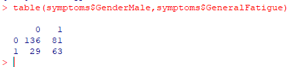
table(symptoms$GenderMale,symptoms$GeneralFatigue)

One problem is that not everyone gave their gender. To make life easier, we can create a new column, “Sex” with this little bit of code. Note that the values are 1 (TRUE) and 0 (FALSE), so we do not need to write ”
symptoms$GenderMale ==1″, instead just “symptoms$GenderMale”

symptoms$sex = ifelse(symptoms$GenderMale,”M”,ifelse(symptoms$GenderFemale,”F”,”U”))

Now we see things better

table(symptoms$sex,symptoms$GeneralFatigue)

We can do the same thing for blood types, i.e.

symptoms$blood_type <- ifelse(symptoms$BloodTypeANegative,”a-“,
ifelse(symptoms$BloodTypeOPositive,”o+”,
ifelse(symptoms$BloodTypeAPositive,”a+”,”U”)))

One of the problems with our data is that often only a few persons provided data. We cannot conclude that only females are o+.

Finding Relationships

Next we are going to look at what groups of symptoms are clustered together. To be more precise — which patients have similar symptoms and thus could be deemed to be a class. This is done by a technique called clustered analysis. This is done by three different method (Complete, Average, Simple). Complete is the recommended approach.

To simplify the code we reload the data and do not add extra columns such as sex or blood type. The lines below computes the normalized distances between every symptoms with each other (240 x 240 computations)

library(tidyverse)

symptoms2 <-read_csv(“http://lassesen.com/ubiome/SymptomsObservations.csv&#8221;)

symptoms.scaled <-dist(scale(symptoms2))

Hierarchical Clustering – Complete

We are clustering people with similar symptoms together and end up with three interesting charts. The charts are on the same data but done in different ways. The number shown on the chart is the observation(person) number in our data.

symptoms.complete <-hclust(symptoms.scaled,method=”complete”)

plot(symptoms.complete)

We can see that people are clustered into groups of similar symptoms

Note that the numbers on the left is the distance that one person is from the next one (shown by the line length).

Patient #47 is sitting by themselves. If you want to see what this person symptoms is, then just enter “str(transpose(symptoms2[47,]))” which will show #47 symptoms (we see that there is a massive number of them – which may be why they are off by themselves)

symptoms.average <-hclust(symptoms.scaled,method=”average”)

plot(symptoms.average, main=”Patients symptoms using average Distance”)

We see that there is almost a progression in symptoms from one person to the next.

symptoms.single <-hclust(symptoms.scaled,method=”single”)

plot(symptoms.single)

Unlike average, everything is one long series and we loose all clusters of similar symptoms.

Reader Playground

The above is a high level “how to do it”. If you want to look only at how a certain group of symptoms are clustered, then it is simple, just add the symptoms you have (you can be explicit in the symptoms you don’t have by using “gender__female == 0”

mysymptoms <- filter(symptoms2, GenderMale, GeneralDepression)

dim(mysymptoms)

we see just 24 rows (other people) and 240 symptoms

Now, let us see what are the odds of some other symptoms, for example, brain fog:

We see that 71% (Mean) with the same symptoms have brain fog. In other words, you can get estimated the probability for symptoms that could be coming up.

Bottom Line

There is much that can be done. The above is just a start. In the next post I will build out a model of relationships between symptoms.

Microbiome Data Science with R

For a year, I have uploaded data uploaded to http://lassesen.com/ubiome/ for interested parties (i.e. data scientists and statisticians) to explore. Making anonymous data available for research has been a key goal for my ubiome site (http://microbiomeprescription.azurewebsites.net ).

In this post, I will document how people can load and so some exploration of it. There are some excellent on line material for learning R, for example dataCamp where the presenters are assistant professors and Ph.D. – but do a clean presentation in their lower level courses.

Getting the data loaded in R

I assume you have installed R or even better, R-Studio (the free one is fine).

I suggest that the following packages are installed:

  1. tidyverse this is a bundle of other packages (the typical ones used by dataCamp)

Now execute (commands are in bold, messages returned in italic):

library(tidyverse)
— Attaching packages ———————————————————————————————————————————————- tidyverse 1.2.1 —
v ggplot2 3.1.0 v purrr 0.3.1
v tibble 2.1.1 v dplyr 0.8.0.1
v tidyr 0.8.3 v stringr 1.4.0
v readr 1.3.1 v forcats 0.4.0
— Conflicts ————————————————————————————————————————————————- tidyverse_conflicts() —
x dplyr::filter() masks stats::filter()
x dplyr::lag() masks stats::lag()
Warning messages:
1: package ‘tidyverse’ was built under R version 3.5.3
2: package ‘tibble’ was built under R version 3.5.3
3: package ‘dplyr’ was built under R version 3.5.3

Next we grab the list of symptoms off the web site and place the data in symptoms

symptoms <-read_csv(“http://lassesen.com/ubiome/Symptoms.csv&#8221;)
Parsed with column specification:
cols(
symptomId = col_double(),
symptom_name = col_character()
)

Next let us inspect the data in symptoms

symptoms
A tibble: 277 x 2
symptomId symptom_name

1 186 Age: 0-10
2 187 Age: 10-20
3 188 Age: 20-30
4 189 Age: 30-40
5 190 Age: 40-50
6 191 Age: 50-60
7 192 Age: 60-70
8 193 Age: 70-80
9 194 Age: 80-90
10 195 Age: 91 and higher
… with 267 more rows

Next we will grab the bacteria taxonomy and place in taxonomy. I cheated to both load and list a portion by putting ( ) around the import. Note that we have the hierarchy included (parent_taxon) as well as the tax_rank.

library(tidyverse)

(taxonomy <-read_csv(“http://lassesen.com/ubiome/Taxonomy.csv&#8221;))
Parsed with column specification:
cols(
taxon = col_double(),
parent_taxon = col_double(),
tax_name = col_character(),
tax_rank = col_character()
)
A tibble: 4,454 x 4
taxon parent_taxon tax_name tax_rank <dbl> <dbl> <chr> <chr>
1 1 0 root root
2 203486 1 Dictyoglomi class
3 4751 1 Fungi kingdom
4 33154 1 Opisthokonta no_rank
5 2 1 Bacteria root
6 2157 1 Archaea superkingdom
7 2759 1 Eukaryota superkingdom
8 1437201 2 Pentapetalae class
9 538999 2 Clostridiales incertae sedis family
10 2323 2 unclassified Bacteria kingdom
… with 4,444 more rows

Next we are going to grab all of the samples available (pre-filtered to “gut” only before I uploaded). Note that is none was detected (0) there is no observation — This means that some of the analysis may need to use NA.

(samples <-read_csv(“http://lassesen.com/ubiome/samples.csv&#8221;))
Parsed with column specification:
cols(
sampleId = col_double(),
taxon = col_double(),
count_norm = col_double()
)
A tibble: 173,356 x 3
sampleId taxon count_norm

1 6 1 1014583
2 6 2 1000000
3 6 237 2614
4 6 712 280
5 6 724 280
6 6 729 280
7 6 815 158414
8 6 816 158321
9 6 818 155
10 6 820 373
… with 173,346 more rows

The last items is the symptoms to sample mixture. Remember that some people do provide symptoms and some people do not. This means that if we are looking at symptoms vs taxonomy (bacteria) — we must restrict observations to only those with symptoms.

(sampleSymptom <-read_csv(“http://lassesen.com/ubiome/SampleSymptom.csv&#8221;))
Parsed with column specification:
cols(
sampleId = col_double(),
symptomId = col_double()
)
A tibble: 8,254 x 2
sampleId symptomId

1 -609 1
2 -609 2
3 -609 3
4 -609 4
5 -609 5
6 -609 6
7 -609 17
8 -609 18
9 -609 19
10 -609 21
… with 8,244 more rows


Simple Manipulations

First we are going to create a data.frame containing only the sampleId of people that have contributed symptoms. Note that we went from
173,356 observations down to 54,632 observations. Roughly 1/3 of the uploads provided symptoms.

(samplesWithSymptoms <- inner_join(samples,sampleSymptom, by=”sampleId”))
A tibble: 54,632 x 4
sampleId taxon count_norm symptomId

1 421 1 1037869 131
2 421 2 1000000 131
3 421 237 3809 131
4 421 543 55 131
5 421 579 55 131
6 421 815 196324 131
7 421 816 196324 131
8 421 818 8480 131
9 421 820 2224 131
10 421 821 109575 131
… with 54,622 more rows

Adding Symptom Names

(samplesWithSymptomNames <- inner_join(samplesWithSymptoms,symptoms, by=”symptomId”))
A tibble: 54,632 x 5
sampleId taxon count_norm symptomId symptom_name

1 421 1 1037869 131 Asymptomatic: No Health Issues
2 421 2 1000000 131 Asymptomatic: No Health Issues
3 421 237 3809 131 Asymptomatic: No Health Issues
4 421 543 55 131 Asymptomatic: No Health Issues
5 421 579 55 131 Asymptomatic: No Health Issues
6 421 815 196324 131 Asymptomatic: No Health Issues
7 421 816 196324 131 Asymptomatic: No Health Issues
8 421 818 8480 131 Asymptomatic: No Health Issues
9 421 820 2224 131 Asymptomatic: No Health Issues
10 421 821 109575 131 Asymptomatic: No Health Issues
… with 54,622 more rows

Adding Taxonomy Information

As above, with Tidyverse, it is a simple one line of code

(samplesExpanded <- inner_join(samplesWithSymptomNames,taxonomy, by=”taxon”))
A tibble: 54,632 x 8
sampleId taxon count_norm symptomId symptom_name parent_taxon tax_name tax_rank

1 421 1 1037869 131 Asymptomatic: No Health Issues 0 root root
2 421 2 1000000 131 Asymptomatic: No Health Issues 1 Bacteria root
3 421 237 3809 131 Asymptomatic: No Health Issues 49546 Flavobacterium genus
4 421 543 55 131 Asymptomatic: No Health Issues 91347 Enterobacteriaceae family
5 421 579 55 131 Asymptomatic: No Health Issues 543 Kluyvera genus
6 421 815 196324 131 Asymptomatic: No Health Issues 171549 Bacteroidaceae family
7 421 816 196324 131 Asymptomatic: No Health Issues 815 Bacteroides genus
8 421 818 8480 131 Asymptomatic: No Health Issues 816 Bacteroides thetaiotaomicron species
9 421 820 2224 131 Asymptomatic: No Health Issues 816 Bacteroides uniformis species
10 421 821 109575 131 Asymptomatic: No Health Issues 816 Bacteroides vulgatus species
… with 54,622 more rows

That’s it for the first post. I will followup with some explorations in coming posts. (If you want to guest write some R analysis posts — write it up as a word document or r-markup file and email to me, ken/at/lassesen.com)

It is my belief that microbiome patterns are more strongly associated with symptoms than ‘official diagnosis’

Bottom Line

Getting the data from the web into R is just a few lines of code (just copy and paste below)

Please pass along to any statisticians or data scientists that you know.

microbiomeprescription site is back up

FYI: Site is back up. There was a tangle of configuration issues with providers that took several days to resolve.

http://microbiomeprescription.com/Data/Symptoms

ME/CFS Symptom List

CFS/ME is not understood by most medical professionals because it lacks:

  • Definitive Tests
  • Definitive Treatment Plans
  • Consistency of presentation from patient to patient for those assigned to this group

One major challenge for front line physicians is they have three patients with similar symptoms, when a fourth one arrives with different symptoms – it throws them into a loop. The CDC and health providers like Kaiser Permanente are slowly working to re-educate physicians (remember it tooks 30 years to re-educate physicians that stomach ulcers were caused by H. Pylori (a bacteria) and not because the person worried too much!). This issue has been made worst from evangelism to MDs of bad science. I like it that the Centers for Disease Control is now emphasising ” Myalgic encephalomyelitis”[pain with inflammation of central nervous system] which should help with changing perceptions. It is matching the neurological classification of ME in the World Health Organization’s International Classification of Diseases (ICD G93.3). 

This is even worst with the general with common misconceptions such as “yuppie flu” and “I get tired too”. In some cases, it has been deemed to be burnout, although a 2019 study found this to be false.

The most common peri-onset events reported by subjects were infection-related episodes (64%), stressful incidents (39%), and exposure to environmental toxins (20%)… At the time of survey, 47% were unable to work and only 4% felt their condition was improving steadily with the majority (59%) describing a fluctuating course. Ninety-seven percent suffered from at least one other illness: anxiety (48%), depression (43%), fibromyalgia (39%), irritable bowel syndrome (38%), and migraine headaches (37%) were the most diagnosed conditions. 

Rates of unemployment can be as high as 81% (7) while ~25% of patients may be homebound or bedridden … the median rate of full recovery is only 5%

Onset Patterns and Course of Myalgic Encephalomyelitis/Chronic Fatigue Syndrome. [2019]

The results indicated that chronic fatigue and burnout should be perceived as 2 distinguishable constructs in the academic context. “

THE RELATIONSHIP BETWEEN CHRONIC FATIGUE SYNDROME, BURNOUT, JOB SATISFACTION, SOCIAL SUPPORT AND AGE AMONG ACADEMICS AT A TERTIARY INSTITUTION [2019]

Last Wednesday, I attended a lunch with the Seattle CFS/ME group. Despite some of the people having had the conditions for over 30 years, now being confined to wheel chairs – the conversation revealed that they were not aware of all of the symptoms (they had some classic CFS symptoms and were not aware that they were CFS associated).

Symptom List

This list (with references) is associated with chronic fatigue syndrome a.k.a.
Myalgic encephalomyelitis. My view is that these diagnosis is a reflection of a microbiome dysfunction. Many CFS patients have gone into temporal full remission from a fecal matter transplant. With this view, we also have a list of symptoms that may be associated with a microbiome dysfunction. This is only a partial list.

Sources: [2015] , [2011] ,[2011] [1987] [1993] [2009]

  • ‘small heart’ with small left ventricular chamber and poor cardiac performance in patient subsets
  • 10% reduction in grey matter volume
  • abdominal pain,
  • abnormal growth factor profiles,
  • air hunger,
  • altered control and reduced cortisol production
  • arthralgias and ‘gelling’ (stiffness),
  • ataxia
  • auditory learning reduced
  • autonomic dysfunction
  • awaken feeling exhausted regardless of duration of sleep,
  • awaking much earlier than before illness onset,
  • bloating,
  • brain stem hypometabolism
  • cardiac and left ventricular dysfunction 
  • cerebrospinal fluid proteomes distinguish patients from healthy controls
  • cervical and/or axillary lymph nodes may enlarge or be tender on palpitation
  • chronic cough(40%),
  • cognitive dysfunction
  • cold extremities
  • day-time sleepiness
  • decreased cortical blood flow
  • decreased natural killer cell signalling and function,
  • decreased neutrophil respiratory bursts and Th1,
  • depression,
  • difficulty processing information
  • extreme pallor or Raynaud’s Phenomenon
  • fatigue of chest wall muscles
  • faucial injection and crimson crescents may be seen in the tonsillar fossae, which are an indication of immune activation.
  • feeling unsteady on feet,
  • Fibromyalgia
  • frequent awakenings,
  • headaches
  • hypoperfusion 
  • immediate recall reduced
  • immune dysfunction
  • impaired depth perception
  • impairment in attention and motor functioning (50%)
  • impairment in speed information processing and executive functioning (40%)
  • inability to focus vision,
  • inability to tolerate an upright position – orthostatic intolerance, neurally mediated hypotension,
  • increases in inflammatory cytokines,
  • insomnia,
  • irritable bowel syndrome
  • Joint hypermobility
  • laboured breathing,
  • light-headedness/dizziness
  • low blood pressure and exaggerated diurnal variation
  • low threshold of physical and mental fatigability (lack of stamina) results in a substantial reduction in pre-illness activity level.
  • marked diurnal fluctuations;
  • marked, rapid physical and/or cognitive fatigability in response to exertion,
  • moons of finger nails may recede.
  • mottling of extremities,
  • muscle weakness,
  • nausea,
  • neuroendocrine and immune symptoms
  • neuroimaging studies report irreversible punctuate lesions
  • neuroinflammation of the dorsal root ganglia
  • nocturia
  • pain,
  • palpitations with or without cardiac arrhythmias,
  • pathological fatigue and malaise that is worse after exertion,
  • photophobia
  • Poor attentional capacity and working memory 
  • poor coordination,
  • postural orthostatic tachycardia syndrome, 
  • pro-inflammatory alleles
  • prolonged sleep including naps,
  • recurrent adenopathy (33%),
  • recurrent feelings of feverishness with or without low grade fever,
  • recurrent low-grade fevers (28%). 
  • recurrent rash (47%), 
  • recurrent sore throat (54%),
  • sensitivity to light, noise, vibration, odor, taste and touch;
  • shift towards a Th2 profile
  • short-term memory loss
  • significant pain can be experienced in muscles, muscle-tendon junctions, joints, abdomen or chest
  • sinusitis,
  • sleeping most of the day and being awake most of the night,
  • slow processing of information 
  • sore throat,
  • subnormal body temperature,
  • susceptibility to viral infections with prolonged recovery periods
  • sustained/switching/divided attention reduced
  • sweating episodes,
  • twitching,
  • unrefreshing sleep
  • urinary urgency or frequency,
  • vivid dreams/nightmares

The COMPASS 31 indicated that 50% have symptoms consistent with orthostatic intolerance. About 43/69 (62%) had Epworth sleepiness scores ≥10, ie, consistent with excessive daytime sleepiness, 26/69 (38%) had significant anxiety and 22/69 (32%) depression measured by HADS A & D. Quality of life is significantly impaired in those with Fukuda criteria CFS (QLS score 64±11) with significant negative relationships between quality of life and fatigue (p<0.0001), anxiety (p=0.0009), depression (p<0.0001) and autonomic symptoms (p=0.04).

Prevalence and characteristics of chronic fatigue syndrome/myalgic encephalomyelitis (CFS/ME) in Poland: a cross-sectional study. [2019]

Bottom Line

I am still in a “flare” dealing with a rollercoaster of the symptoms above. Most patients when ask for symptoms will give a list of 3-4 only. If you walk these patients thru the above list, the numbers increase — often to several dozens — the symptoms listed are the worst ones and the other ones tend to be ignored. I do not have just one or two of the above, but a pretty good list when waxes and wanes throughout each day.

For myself, when in a flare, I will enumerate the list and then “cherry pick” active symptoms looking at the audience who will be hearing it. Often patients will just list they dominant symptoms, “tiredness, sore throat” etc which will often be interpreted by others as low significance.

For example, instead of the wordy “Postural orthostatic tachycardia syndrome (POTS)” I would simply say tachycardia (verified by a pulse of 170 on my monitoring smart watch). A simple neurological symptoms usually go over better than “slow mental processing”, “mental fatigue”. If someone presses more, I will respond with I have ”
“hypoperfusion in the brain – my brain is not getting enough oxygen” or more technical “hypoperfusion in the brain according to SPECT Brain Scans”. I know of CFS patients that have had transient ischemic attack (TIA), especially after a stressful event.

Of course, the problem is having diminished executive decision abilities — so patients make poor presentation of their symptoms to others 😦

Another trigger of microbiome shifts: stroke, and ?WiFi?

The model that I am assuming for conditions like CFS, is some event triggers a microbiome shift which persists in a dysfunctional state. A few of these events are well known, or suspected:

  • Infection (viral or bacteria) – best documented example is Bergen Norway – giardiasis
  • Stress:
    • ” an integrative conceptual model is proposed in which stress-induced enteric dysbiosis and intestinal permeability confer risk for negative mental health outcomes through immunoregulatory, endocrinal, and neural pathways.  ” [2017]
    • PTSD (Articles)
  • Vaccinations – in theory should, no studies done on microbiome shifts before and after vaccination (yet!). If the vaccination works, it has been shown that depends on the microbiome being right [2017]
  • Antibiotics or antivirals

In reviewing a news article, The fascinating effect a stroke has on the gut microbiome, reporting on the International Stroke Conference

Prior research from the same team revealed a stroke does have an immediate effect on the microbiome, but how long these effects last for was not known. Using animal models the researchers conducted microbiome examinations three days, two weeks and four weeks following an induced stroke…. A notable decrease was seen in Bifidobacteriaceae, a common bacteria found in probiotics, up to four weeks past the stroke, while increases were seen in Helicobacteraceae across the same observational period.

Another intriguing change in the gut seemingly brought on by the stroke were notable abnormalities in intestinal tissue. Normally in healthy animal models this tissue appears structured in orderly ways, almost like branches of coral. However, close examination up to four weeks post-stroke revealed the villi, structures that project off the intestinal wall, were scrambled and visibly quite different from the healthy models.

The fascinating effect a stroke has on the gut microbiome,

The real interesting aspect of the article was:

Another compelling study from 2017 suggested magnetic simulation to specific areas in the brain can affect the composition of a person’s gut microbiome.

The fascinating effect a stroke has on the gut microbiome,

The question is then — do cell phones create magnetic fields (that could potentially stimulate the brain). The answer is yes:

Among the valves tested, the settings of the Strata valve, the Hakim valve, and the Sophy valve were affected by magnetic flux densities of 6.0, 17.5, and, 40.0 mT, respectively. Cell phones produce a magnetic flux density of 3.0 to 40.0 mT. 

Effect of cell phone magnetic fields on adjustable cerebrospinal fluid shunt valves [2005]

And for Wifi, the evidence is cleaner still:

The pure cultures of Listeria monocytogenes and Escherichia coli were exposed to RF-EMFs generated either by a GSM 900 MHz mobile phone simulator and a common 2.4 GHz Wi-Fi router. It is also shown that exposure to RF-EMFs within a narrow level of irradiation (an exposure window) makes microorganisms resistant to antibiotics

Evaluation of the Effect of Radiofrequency Radiation Emitted From Wi-Fi Router and Mobile Phone Simulator on the Antibacterial Susceptibility of Pathogenic Bacteria Listeria monocytogenes and Escherichia coli. [2017]

Bottom Line

While we know that all of the above can cause microbiome shifts, most people microbiome returns to normal. Most people. As a statistician, I know that as the number of low risk events increases, the chance of a significant event cumulates.

We cannot say: Wifi, vaccination etc causes any specific long term autoimmune conditions, it just increases the risk — like smoking does. There are people who seem immune to the effects of smoking (like the Comedian George Burns who lived to 100 and love smoking cigars).